
Time Series Analysis: Part 1
Published:
- Kerui Yang
- Share on
- You May Also Enjoy
- Time series analysis using XGBoost
- Data Cleaning
- Train Test Split
- Feature Creation
- Visalising Feature / Target Relationship
- Model Creation
- Extracting Feature Importance
- Forecasting
- Model Analysis
Time series analysis using XGBoost
import pandas as pd
import numpy as np
import seaborn as sns
import matplotlib.pyplot as plt
import xgboost as xgb
from sklearn.metrics import mean_squared_error as mse
# OS
from pathlib import Path

# Styling
color_pal = sns.color_palette("Set2")
plt.style.use('seaborn-v0_8-colorblind')
data_path = Path('data/PJME_hourly.csv')
df = pd.read_csv(data_path)
df.info()
<class 'pandas.core.frame.DataFrame'>
RangeIndex: 145366 entries, 0 to 145365
Data columns (total 2 columns):
 #   Column    Non-Null Count   Dtype
---  ------    --------------   -----
 0   Datetime  145366 non-null  object
 1   PJME_MW   145366 non-null  float64
dtypes: float64(1), object(1)
memory usage: 2.2+ MB
df.head()
| Datetime | PJME_MW | |
|---|---|---|
| 0 | 2002-12-31 01:00:00 | 26498.0 |
| 1 | 2002-12-31 02:00:00 | 25147.0 |
| 2 | 2002-12-31 03:00:00 | 24574.0 |
| 3 | 2002-12-31 04:00:00 | 24393.0 |
| 4 | 2002-12-31 05:00:00 | 24860.0 |
df.tail()
| Datetime | PJME_MW | |
|---|---|---|
| 145361 | 2018-01-01 20:00:00 | 44284.0 |
| 145362 | 2018-01-01 21:00:00 | 43751.0 |
| 145363 | 2018-01-01 22:00:00 | 42402.0 |
| 145364 | 2018-01-01 23:00:00 | 40164.0 |
| 145365 | 2018-01-02 00:00:00 | 38608.0 |
Data Cleaning
Steps undertaken:
- set index
- typecast
df.set_index('Datetime', inplace=True)
df.index = pd.to_datetime(df.index)
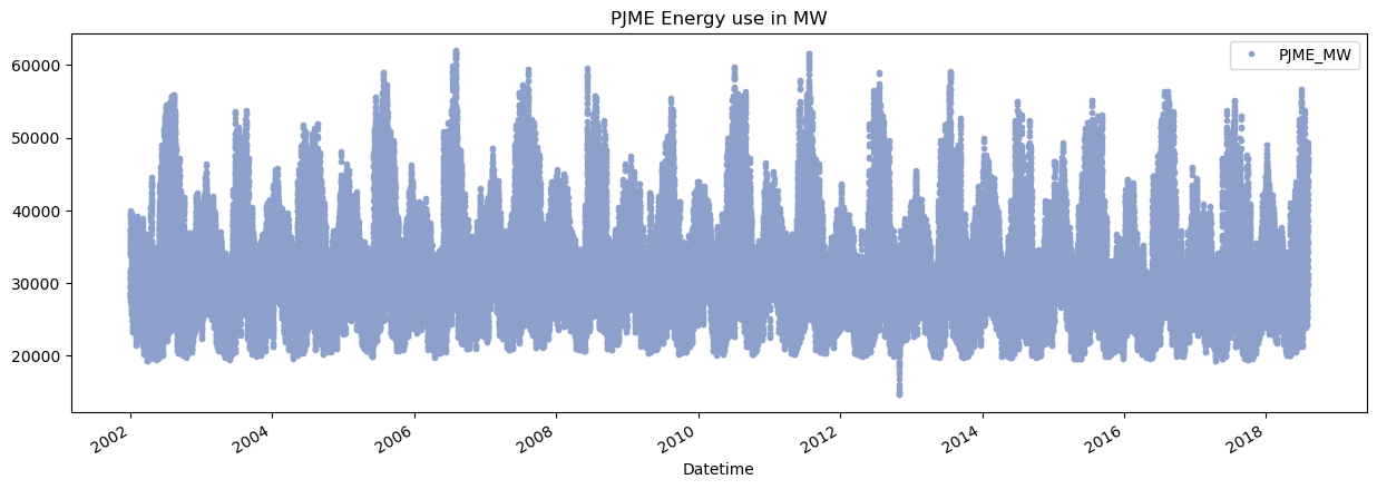
df.plot(title='PJME Energy use in MW',
        style='.',
        figsize=(15,5),
        use_index=True,
        color=color_pal[2])
plt.show()
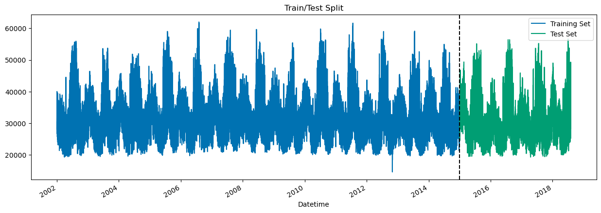
Train Test Split
train = df.loc[df.index < '01-01-2015']
test = df.loc[df.index >= '01-01-2015']
fig, ax = plt.subplots(figsize=(15,5))

train.plot(ax=ax, label='Train', title='Train/Test Split')
test.plot(ax=ax, label='Test')
ax.axvline('01-01-2015', color='black', ls='--')
ax.legend(['Training Set', 'Test Set'], loc='upper right')
plt.show()
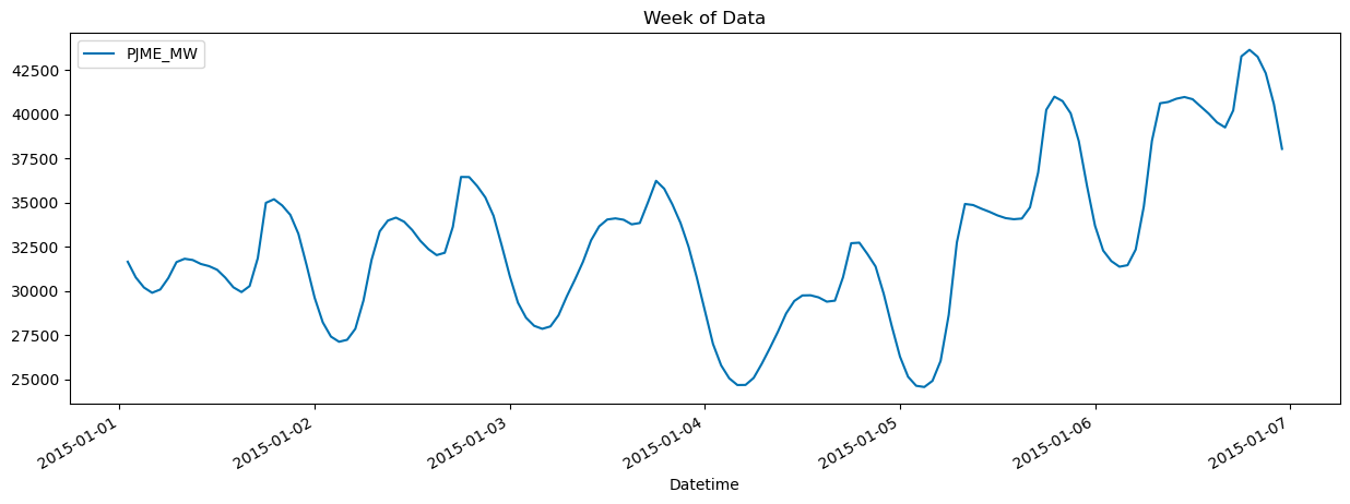
# visualising one week
df.loc[(df.index >'01-01-2015') & (df.index < '01-07-2015')] \
    .plot(figsize=(15,5), title='Week of Data') # note & denotes element-wise logical, whereas 'and' will ask python to typecast into bool
<Axes: title={'center': 'Week of Data'}, xlabel='Datetime'>
Feature Creation
def create_features(df):
    """
    Create time series features given df with datetim index
    """
    df = df.copy()
    df['hour'] = df.index.hour
    df['dayofweek'] = df.index.dayofweek
    df['quarter'] = df.index.quarter
    df['month'] = df.index.month
    df['year'] = df.index.year
    df['dayofyear'] = df.index.dayofyear
    df['dayofmonth'] = df.index.day
    df['weekofyear'] = df.index.isocalendar().week
    return df
df = create_features(df)
Visalising Feature / Target Relationship
df.columns
Index(['PJME_MW', 'hour', 'dayofweek', 'quarter', 'month', 'year', 'dayofyear',
       'dayofmonth', 'weekofyear'],
      dtype='object')
Generating a heatmap of correlations, and the correlation with the target variable.
corr = df.corr()
fig, (ax1, ax2) = plt.subplots(ncols=2, figsize=(15, 5))
fig.subplots_adjust(hspace=-0.5, top=0.9, left=0.1)
ax1 = sns.heatmap(
    corr,
    vmin=-1, vmax=1, center=0,
    cmap=sns.diverging_palette(20, 220, n=200),
    square=True,
    ax = ax1
)
ax1.set_xticklabels(
    ax1.get_xticklabels(),
    rotation=45,
    # horizontalalignment='right'
)
ax1.set_title('Correlation Heatmap')

# plotting correlation with target
corr_target = df.corr()[['PJME_MW']].sort_values(by=['PJME_MW'],ascending=False)
ax2 = sns.heatmap(corr_target,
                  vmin=-1, vmax=1,
                  cmap=sns.diverging_palette(20, 220, n=200),
                  square=True,
                  cbar=False,
                  ax=ax2)
ax2.set_title('Correlation with PJME_MW, descending');
plt.tight_layout()
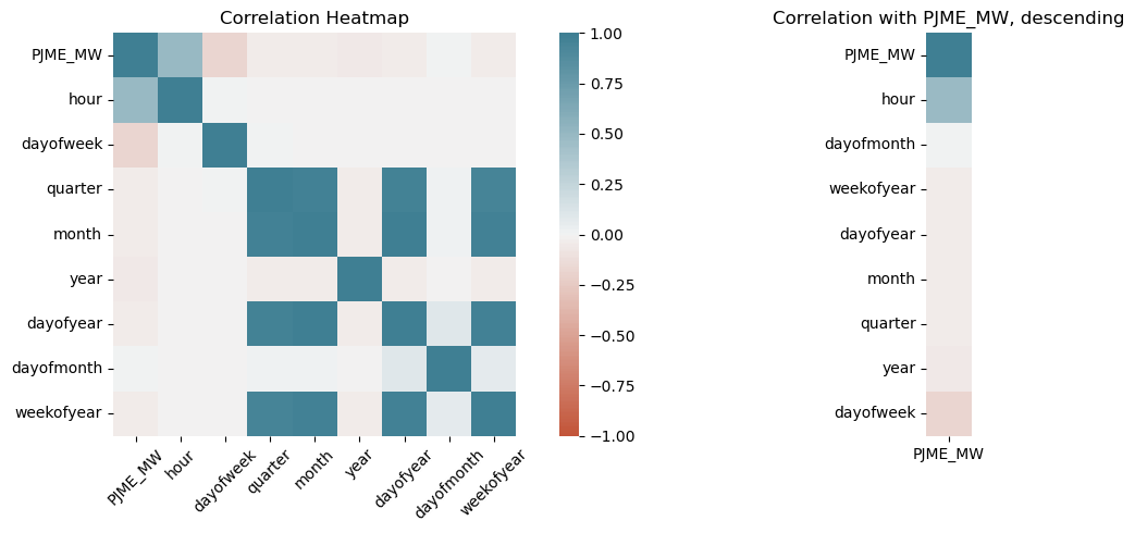
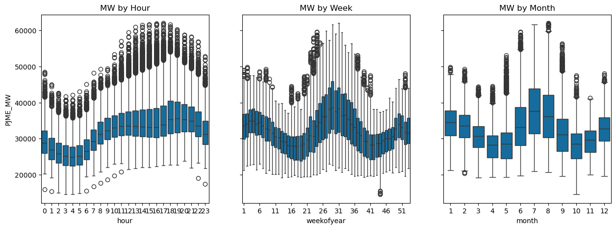
We can see that the most strongly correlated variable is hour, followed by day. Lets visualise this below:
fig, (ax1, ax2, ax3) = plt.subplots(ncols=3, figsize=(15, 5), sharey=True)
sns.boxplot(data=df, x='hour', y='PJME_MW', ax=ax1)
ax1.set_title('MW by Hour')

sns.boxplot(data=df, x='weekofyear', y='PJME_MW', ax=ax2)
ax2.set_title('MW by Week')
# Set ticks every 4 week
ax2.xaxis.set_major_locator(plt.MaxNLocator(12))

sns.boxplot(data=df, x='month', y='PJME_MW', ax=ax3)
ax3.set_title('MW by Month');
Model Creation
train = create_features(train)
test = create_features(test)

FEATURES = ['dayofyear', 'hour', 'dayofweek', 'quarter', 'month', 'year']
TARGET = 'PJME_MW'

X_train = train[FEATURES]
y_train = train[TARGET]

X_test = test[FEATURES]
y_test = test[TARGET]
reg = xgb.XGBRegressor(base_score=0.5, booster='gbtree',
                       n_estimators=1000,
                       early_stopping_rounds=50,
                       objective='reg:linear',
                       max_depth=3,
                       learning_rate=0.01)
reg.fit(X_train,y_train,
        eval_set=[(X_train,y_train), (X_test, y_test)],
        verbose=200)
[0]	validation_0-rmse:32605.13970	validation_1-rmse:31657.15729


/home/kyan/miniforge3/lib/python3.10/site-packages/xgboost/core.py:160: UserWarning: [07:02:00] WARNING: /home/conda/feedstock_root/build_artifacts/xgboost-split_1713397688861/work/src/objective/regression_obj.cu:209: reg:linear is now deprecated in favor of reg:squarederror.
  warnings.warn(smsg, UserWarning)


[200]	validation_0-rmse:5837.33066	validation_1-rmse:5363.58554
[400]	validation_0-rmse:3447.54638	validation_1-rmse:3860.60088
[600]	validation_0-rmse:3206.55619	validation_1-rmse:3779.04119
[800]	validation_0-rmse:3114.34038	validation_1-rmse:3738.38209
[989]	validation_0-rmse:3059.85847	validation_1-rmse:3727.94591
XGBRegressor(base_score=0.5, booster='gbtree', callbacks=None,
             colsample_bylevel=None, colsample_bynode=None,
             colsample_bytree=None, device=None, early_stopping_rounds=50,
             enable_categorical=False, eval_metric=None, feature_types=None,
             gamma=None, grow_policy=None, importance_type=None,
             interaction_constraints=None, learning_rate=0.01, max_bin=None,
             max_cat_threshold=None, max_cat_to_onehot=None,
             max_delta_step=None, max_depth=3, max_leaves=None,
             min_child_weight=None, missing=nan, monotone_constraints=None,
             multi_strategy=None, n_estimators=1000, n_jobs=None,
             num_parallel_tree=None, objective='reg:linear', ...)
In a Jupyter environment, please rerun this cell to show the HTML representation or trust the notebook. On GitHub, the HTML representation is unable to render, please try loading this page with nbviewer.org.
XGBRegressor(base_score=0.5, booster='gbtree', callbacks=None,
colsample_bylevel=None, colsample_bynode=None,
colsample_bytree=None, device=None, early_stopping_rounds=50,
enable_categorical=False, eval_metric=None, feature_types=None,
gamma=None, grow_policy=None, importance_type=None,
interaction_constraints=None, learning_rate=0.01, max_bin=None,
max_cat_threshold=None, max_cat_to_onehot=None,
max_delta_step=None, max_depth=3, max_leaves=None,
min_child_weight=None, missing=nan, monotone_constraints=None,
multi_strategy=None, n_estimators=1000, n_jobs=None,
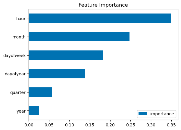
num_parallel_tree=None, objective='reg:linear', ...)Extracting Feature Importance
fi = pd.DataFrame(data=reg.feature_importances_,
                  index=reg.feature_names_in_,
                  columns=['importance'])
fi.sort_values('importance').plot(kind='barh', title='Feature Importance')
plt.show()
Forecasting
# predict on test data
test['prediction'] = reg.predict(X_test)
# merging with the df and the test dataset
df = df.merge(test[['prediction']], how='left', left_index=True, right_index=True)
ax = df_merged[['PJME_MW']].plot(figsize=(15,5))
df_merged['prediction'].plot(ax=ax, style='.', label='Prediction')
plt.legend(loc="upper right")
ax.set_title('Prediction vs Truth');
---------------------------------------------------------------------------

NameError                                 Traceback (most recent call last)

Cell In[22], line 1
----> 1 ax = df_merged[['PJME_MW']].plot(figsize=(15,5))
      2 df_merged['prediction'].plot(ax=ax, style='.', label='Prediction')
      3 plt.legend(loc="upper right")


NameError: name 'df_merged' is not defined
df_merged.loc[(df_merged.index >'01-01-2015')][['PJME_MW', 'prediction']] \
    .plot(figsize=(15,5), title='Predictions vs Truth');
Showcasing one weeks worth of data:
df_merged.loc[(df_merged.index >'01-01-2017') & (df_merged.index < '01-07-2017')][['PJME_MW', 'prediction']] \
    .plot(figsize=(15,5), title='Week of Data') # note & denotes element-wise logical, whereas 'and' will ask python to typecast into bool
Notes:
- Models data quite well, up / down trends per day, including nighttime usage
- Does not model peaks / troughs well
Future improvements:
- Model days of year e.g. holidays
- Add more features
- more robust cross validation
Model Analysis
Showcasing the best and worst performing results
score = np.sqrt(mse(test[TARGET], test['prediction']))
print(f'RMSE Score on test set: {score:.4f}')
Error calculation
test['error'] = np.abs(test[TARGET] - test['prediction'])
test['date'] = test.index.date
Finding the best and worst performing days
Worst Performing Days:
test.groupby(['date'])['error'].mean().sort_values(ascending=False).head(3)
Best performing days:
test.groupby(['date'])['error'].mean().sort_values(ascending=True).head(3)
The best performing days was in october 2017, and all best -performing days were in october. The worst performing days were in august 2016.
Lets visualise this:
fig, (ax1, ax2) = plt.subplots(ncols=2, figsize=(15, 5), sharey=True)
df.loc[(df.index >'08-07-2016') & (df.index < '08-27-2016')][['PJME_MW', 'prediction']].plot(ax=ax1)
df.loc[(df.index >'10-20-2017') & (df.index < '11-07-2017')][['PJME_MW', 'prediction']].plot(ax=ax2);
We can see that we consistently underpredicted for a period of time in august 2016, and some investigation is necessary to determine why that was the case.